
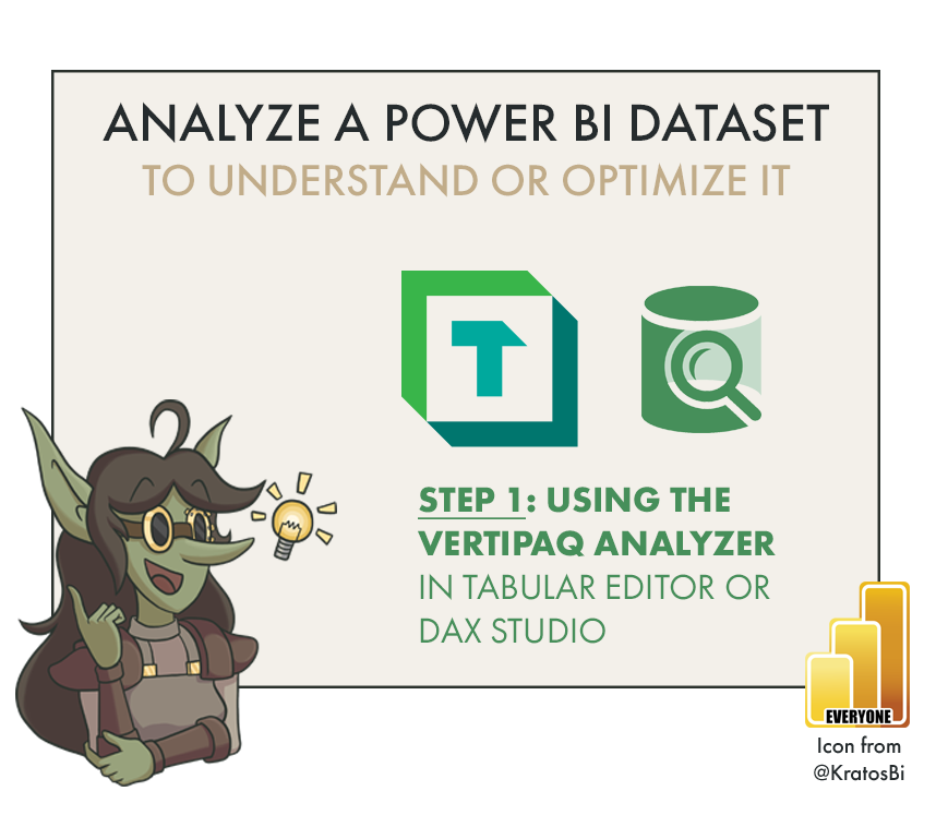
Analyze a Dataset with Tabular Editor 3 - VertiPaq Analyzer
ONE OF THE BEST & EASIEST TOOLS TO ANALYZE A DATASET
…learn why you need to be using VertiPaq Analyzer in Tabular Editor 3 or DAX Studio 3
In this series, we will learn how to effectively assess an existing or ‘inherited’ dataset.
We will learn how to…
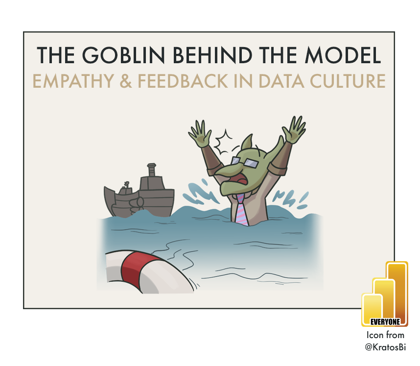
Remember the person behind the model
Conduct an efficient analysis with Tabular Editor 3Analyze the model with VertiPaq Analyzer
Explore the model with Dynamic Management Views (DMVs)
Automate DMVs execution with C# scripts in Tabular Editor
Before we start, it is assumed that…
You have installed Tabular Editor 3 (TE3) and DAX Studio.
You have downloaded the VertiPaq Analyzer from sqlbi
You have a dataset to analyze
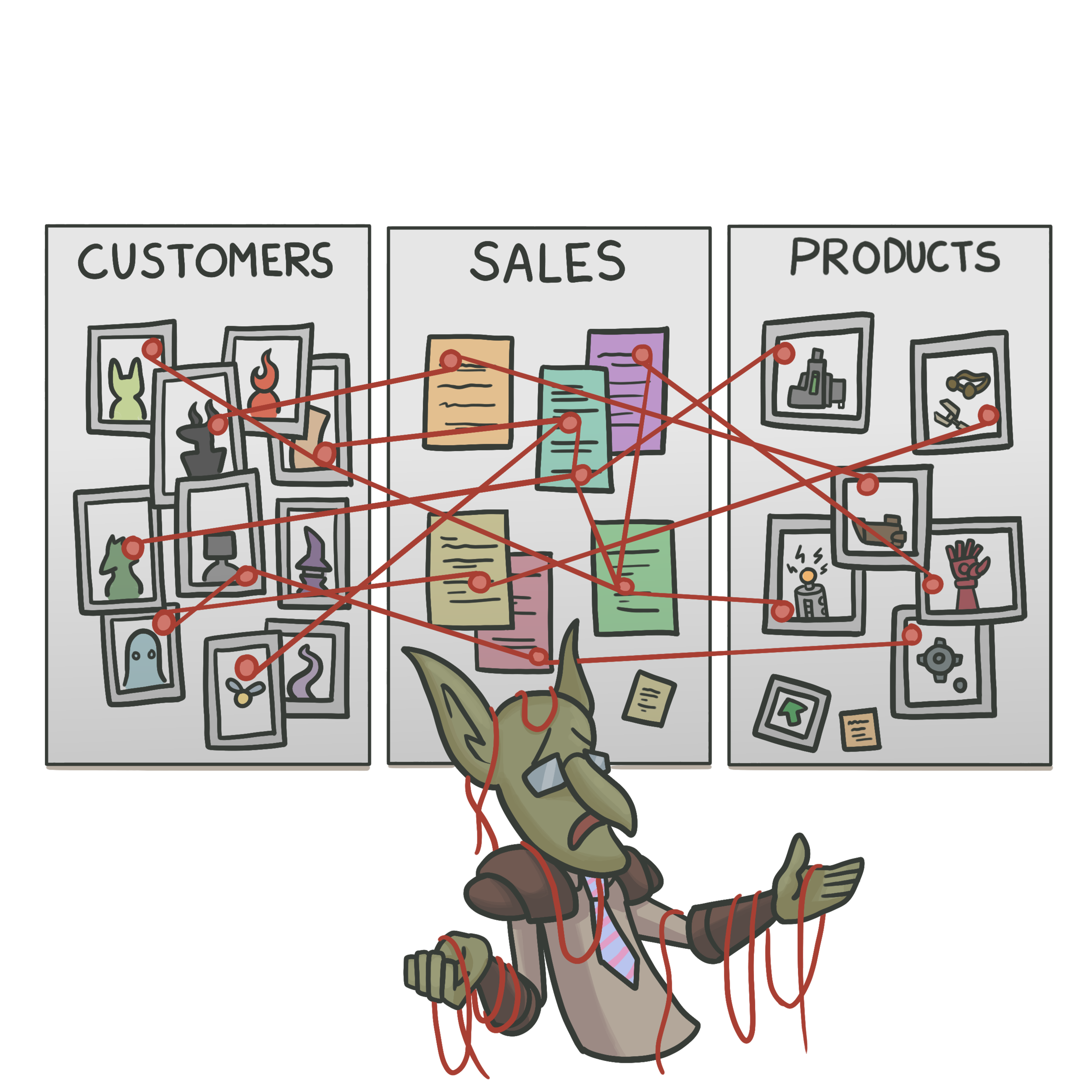
Inheriting a dataset

Working with a dataset you did not create is challenging.
There is rarely documentation that gives a good overview of the scope, logic and shortcomings of the dataset, necessitating deep dives into the model itself in order to understand it. This is particularly true when inheriting problem models that you need to “fix”, perhaps plagued by performance issues, inaccurate calculations, or absent functionality. It’s essential to be thorough in these investigations, but at the same time to also be efficient and objective in the analysis.
In this series, we look at how to handle “model inheritance”, with particular focus on how Tabular Editor 3 makes this very easy & efficient. In this article, we look at why using the VertiPaq Analyzer - integrated in TE3 & DAX Studio - should be your first step when analyzing another dataset.
Describe your models and find easy optimization steps with this valuable tool.

Using the VertiPaq Analyzer to find optimizations that reduce dataset size by 70% after just 1 hour of work. At the bottom of the article is a step-by-step of this analysis.
Part 2: Tabular Editor 3 & The VertiPaq Analyzer
What is the VertiPaq Analyzer & why is it useful?
Tabular Editor 3 (TE3) is an extremely powerful tool for developing tabular data models. Among the many features present in TE3 are those which let you browse the data model metadata and contents very easily. When opening another model for the first time, one of these tools comes particularly in handy, and should always be your first go-to option: The VertiPaq Analyzer.
Below a video of a presentation from Marco Russo at sqlbits 2021 introducing VertiPaq Analyzer

VertiPaq Analyzer
The VertiPaq Analyzer is not something intrinsic to TE3 itself, but rather another tool integrated inside TE3. If you have worked with DAX Studio before, you might already be familiar with the VertiPaq Analyzer, as it’s integrated there in a similar fashion. Created by sqlbi, the VertiPaq Analyzer is an analytical tool for tabular models, which gathers precise and useful summary statistics about the model contents. The name is from the VertiPaq engine, the technology used in tabular models like your Power BI dataset to store & query data.
A prominent use-case for the VertiPaq Analyzer is optimizing model size and referential integrity (RI) of relationships (more on that, below). The kind of information gathered by the Analyzer pertains to the different objects present in a dataset and the in-memory storage size they occupy. This is relevant and useful because the size of a data model is often proportional to its performance, both in terms of refresh and query times; if you want fast reports and up-to-date data, optimizing dataset size is a key step to getting there. Using the VertiPaq Analyzer one can, for example, quickly identify tables and columns with a high cardinality that are taking disproportionate space in the dataset, and can consider actions to change or remove the column to optimize dataset size.
Without documentation, things get messy
VertiPaq Analyzer isn’t only useful for analytical purposes, but also descriptive ones; it’s handy for generating meaningful documentation about the model. If you need a list of all the in-memory objects and their size, this is the fastest way to produce it. The results from the VertiPaq analyzer can be exported as a .vpax file, for later viewing in DAX Studio, Tabular Editor 3 or the VertiPaq .xlsm pivot table from sqlbi.
The analyzer gets this information using the Dynamic Management Views (DMVs) that exist in every analysis services server and database, including for Power BI datasets when we connect to a local instance or via XMLA endpoint to the service. These views can be queried to get aggregate or detailed information, not only the model and its contents, but also about the users connecting to it, and what they are doing. You can query these DMVs yourself from Tabular Editor 3 and DAX Studio using a limited, SQL-like syntax, but we’ll discuss that further in the next article of this series. For now, all you need to know is that the VertiPaq Analyzer does this for you, saving you time and returning relevant, valuable information for you to analyze the dataset.
We now know what the VertiPaq Analyzer is. But how do we use it, and the data it produces?
How to use the VertiPaq Analyzer from TE3
Step 1: Connect to the model from TE3
Open TE3 and connect to the model. If you have Premium Capacity or the model is hosted on a Premium-Per User workspace, you should ‘Load model from database’ by connecting to the dataset via the XMLA Endpoint. If you have only a Pro environment or want to analyze a local .pbix, the file needs to be open from Power BI Desktop. You can then connect in a similar way, but selecting instead the “Local instance”.

Load the model from database
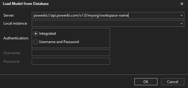
Enter the XMLA endpoint in “server” for premium or select the Local instance if you connect to a .pbix
Step 2: Save a copy of your model metadata
Since TE3 is a read/write tool, you want to make a copy of your model metadata in case you accidentally change anything. When opening another model for the first time, this is a good practice. From TE3, save the database.json folder structure. If you have a Premium or PPU capacity, you should then connect to this folder structure and a Power BI workspace using TE3’s workspace mode, deploying the dataset to a space where you can safely explore it without affecting anyone else. If you are unfamiliar with the TE3 save formats and workspace mode, I have previously written an article about how to do it, available here.

Step 3: Open the VertiPaq analyzer tab & click ‘Collect Stats’
This will run the VertiPaq analyzer over your model. It’s as simple as pushing a single button. The hard part is reading and interpreting the data you get back, if you don’t know what you are looking for!
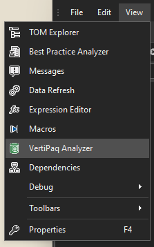
Access from the ‘View’ menu
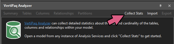
Run the VertiPaq Analyzer on the model
Step 4: Browse the data
The results returned by the VertiPaq analyzer are organized into 5 tabs:
VertiPaq Summary of the dataset
Local dataset .pbix
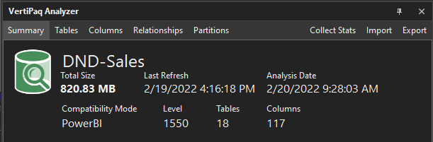
1. Summary:
This is a high-level overview of the model, telling you its total size, as well as the number of tables and columns. The last refresh datetime of the model is visible, as is that of the analysis. The compatibility mode and level describes the type & version of the dataset.
Note 1 - Why does the “Total Size” of the VertiPaq Analyzer not correspond to the .pbix file size?
The ‘total size’ from the VertiPaq Analyzer results does not correspond to the compressed size of the .pbix on disk; it will be larger. This is because a .pbix file is actually a .zip format, which applies a more efficient compression of the in-memory data and thus a smaller size of the .pbix. You can thus think of the VertiPaq Analyzer result as the “true size” of the compressed, in-memory data in the dataset, and not the filesize of the .pbix.
Note 2 - OK but the model is bigger than I expected - why?
The model may appear larger after a refresh. After performing a ‘process’ operation (model refresh or ‘calculate’ process of - for example - calculated tables with dependencies), the VertiPaq engine allocates 1MB of memory to the column dictionary. This is not visible when i.e. opening a .pbix without refreshing the data.
Source: An article about this from sqlbi.
Note 3 - Why does the Analysis Date not correspond to my local datetime?
The refresh & analysis datetime will be dependent on the server time if you are connected to a dataset via XMLA endpoint. In the above example, the analysis was done at 10:28 CET, which corresponds to 09:28 UTC.
The Tables Tab: Click to enlarge the image
2. Tables:
This tab provides summary statistics about all the tables in the data model. It’s a matrix that can be expanded & collapsed to view the columns beneath. The columns can also be seen without their parent tables in the ‘Columns’ tab. In all of the tabs, you sort the columns, re-arrange column order, and filter to specific values in the TE3 table UI.
Note - When I expand the tables, I see a “Row Number” column. What’s that?
This represents the (Blank) row that is created when an Unknown member is detected, due to a referential integrity (RI) violation in a relationship. Every table has this (Blank) row for these scenarios. For more about RI violations, see the respective drop-down menu, below:
Definitions adapted from the sqlbi article here
Each of the below terms is a field in the ‘Table’ view. Click to expand for more info.
-
The maximum number of unique values in any given column of the table. The cardinality will be proportional to the total size of the object.
-
The total size of the table in memory, in bytes; includes all objects.
Table Size =
Relationships
+ Dictionary
+ Data
+ Column hierarchies
+ User hierarchies -
The total size of the column in memory, in bytes; includes multiple objects.
Column Size =
Dictionary
+ Data
+ Column hierarchies -
The total size of the compressed data in-memory.
-
The total size of the dictionary structure.
What is a dictionary?
The dictionary is an indexation of distinct values for a column, known as HASH encoding. The details of the VertiPaq engine go beyond the scope of this article, but put simply -
For HASH encoding, VertiPaq stores distinct values of a column as an integer index, which experiences more optimal compression. To get the original values, it just has to match the index to the values it replaced (key:value dictionary pairing).
For a good summary see this YouTube video by sqlbi and this article by Data Mozart.Note:
As mentioned above, you should be cautious about measuring the dictionary size after a process operation (refresh), as it will be larger. This includes changing a calculated table expression or performing an action that will refresh the model metadata. Instead, run VertiPaq Analyzer immediately after opening the .pbix file. -
The total size of the column hierarchies automatically created.
-
The column encoding type.
Many: Typically the value shown for the table. Includes both HASH & VALUE
HASH: Typically unsummarized, group-by columns (dimensions) and foreign keys. HASH encoding results in the creation of a dictionary.
VALUE: Summarized, aggregable values (facts). VALUE encoded columns typically don’t have a dictionary.Note:
The encoding type is selected by VertiPaq, automatically. However, for some columns, it may be worthwhile to check whether the most optimal choice has been made. It is possible, for example, that a document number field is treated with HASH encoding, when VALUE encoding may lead to more optimal compression. In Tabular Editor, you can change the “Encoding Hint” of the Column, under “Properties”, and test the effect on the column size.
Please check out this nice summary article by Data Mozart here. -
Data Type of the column
Boolean: True/False
Int64: Integer (64-bit; 32 and 16-bit integers don’t exist in tabular models)
Double: Decimal number
Fixed: Fixed point decimal
String: Text fields
DateTime: Date and time data
Date: Date data
Time: Time data -
The number of relationships from that table that have referential integrity violations.
What is Referential Integrity?
Referential Integrity (RI) in a Power BI dataset is a property of relationships. RI assumes values from the ‘many’ side of a relationship (usually the fact table) should be present in the values of the column on the ‘one’ side (usually the dimension table). This is because at query evaluation, an extended table is created from the one to the many side, using LEFT OUTER JOIN semantics on the ‘one’ side table. Thus RI violation rows - or unmatched foreign keys - result in the creation of an Unknown member, grouping by (Blank) values that you will see in visuals, slicers and filters.Why is Referential Integrity important?
Removing RI violations from your model will not only result in filters and slicers no longer having (Blank) values. According to this article by Phil Seamark, it also can have a performance impact on your reports, resulting in more optimized queries when removed. -
The hierarchy created by users in the Power BI Desktop UI.
-
The relative size of columns in a given table (% of grand total) which easily allows the identification of abnormally large columns that could be adjusted or removed from the dataset for optimization.
-
The relative size of the object (Table or Column) in the database (% of grand total). This easily allows the identification of a problem child which is disproportionately large compared to other objects.
-
The number of segments in the table rowset. The default segment size in Power BI is 1 million rows, but in models with large dataset storage mode enabled, is 8 million rows.
What is a segment?
Segments refer to how VertiPaq compresses and queries data. When processed, the VertiPaq engine will not read and compress the entire partition at once, but rather break the operation up into segments to parallelize. Once read, the first segment will be compressed, while in parallel the VertiPaq engine will read the next segment.Why are segments important?
For big datasets, larger segment sizes can result in more optimal compression. However, this can also impact query performance, as having more segments means that at query time, more parallel operations are required to execute the query on the compressed data.For a more in-depth explanation, check this article by sqlbi.
-
A count of the number of partitions in the table.
What is a partition?
A partition is a logical segmentation of the data in the table (rowset). In Power BI, this is usually observed in the context of incremental refresh. There, data is partitioned using datetime fields and parameters. The benefit of this is that a refresh policy can be set to only conduct a data process of specific partitions, resulting in faster refresh times if, for example, you wish to only refresh data in the last month. However, it is also possible to partition data using other dimensions. -
A distinct count of the number of columns in the table.
The Columns Tab: Click to enlarge the image
3. Columns:
This view is effectively the same as the table view, but drilled down to the columns only. There’s no information about referential integrity of relationships per table. This columnar view lets you look independently of tables to see which columns are taking abnormal amount of space.
The Relationships Tab: Click to enlarge the image
4. Relationships:
This view shows information about all the relationships in the dataset. For each relationship you see the cardinality of the “to” and “from” columns, the combination of which determines the size of the relationship. If there is a high cardinality on the ‘from’ column that is not present on the ‘to’ column, it might suggest superfluous data in the dimensions table that could be removed.
The most important columns, though, are the last three, which provide more detailed information about the referential integrity violations.
Video from sqlbi
Each of the below terms is a field in the ‘Relationships’ view not in the previous views. Click to expand for more info.
-
If there exists a referential integrity (RI) violation, it means that there are missing keys on the ‘from’ side of the relationship that are present in the ‘to’ side.
This column shows for each relationship the distinct count of missing keys on the ‘to’ side, so you know the extent of the RI violation for that relationship.
-
While the ‘missing keys’ provides the distinct count of values that are absent on the ‘from’ side but present on the ‘to’ side, this column gives the total row count; it illustrates the impact of the RI violation on the ‘from’ table.
-
A representative sample of the missing keys. Shows the minimum, median & maximum values missing on the ‘from’ side.
Why is this valuable?
Once you understand if there is an RI violation and the extent that it is impacting the relationship, the most actionable information for you is to know which keys are missing. You can then examine your ETL for these keys in order to understand in which step they disappear and resolve the issue. Or, if it is a master data problem, immediately provide those examples to the appropriate stakeholders.
The Partitions Tab: Click to enlarge the image
5. Partitions:
This view is focused specifically on the data loaded into the model and understanding how it is stored and compressed. What is unique, here, is that you can expand a table to examine the various partitions beneath it. This might be interesting if you have a large table consisting of many partitions, and are trying to understand whether there are optimizations to that table that could be made, i.e. by changing how it is partitioned.
For example, if you have 5 years of data, partition the data by month, and have about 1M rows per month, you have ±60M rows of 60 partitions and 60 segments. In that case, you would not benefit from enabling Large Dataset storage mode, which increases segment size to 8M rows. You might decide instead based on this information to partition your data by year and enable the large model storage, so you have less partitions but larger - and therefore also fewer - segments, which could have a positive impact on how your data is compressed.
Step 5: Our Investigation Tree: Exploring the Data
Now that we’ve collected and understood the data, we need to interpret what it could mean for the dataset we are investigating. Usually, we want to find outliers or unique aspects of the dataset or data that we should be aware of.
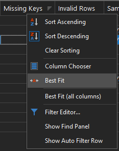
Note - Right-clicking on the table in TE3 gives a lot of filtering & sorting options:
If you are looking at a specific subset of data or analysis results, you can drag & drop columns to rearrange, make text bigger with CTRL + mouse wheel up, or sort & filter results to your liking. TE3 has a fantastic UI for doing specific filtering to restrict results to what you want to look at.
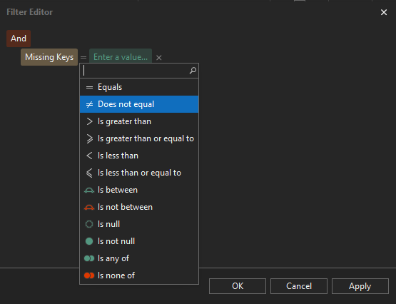
The TE3 filter editor in the table UI lets you limit results to exactly what you want.
EXAMPLE CASE STUDY
Now that we understand the results, let’s take a look at some questions for our dataset:

Dataset we are analyzing - 821 MB to start
1. Do we see unexpected or hidden columns, for example, auto-Date tables?
If you have auto date-time enabled in Power BI Desktop, it creates a hidden date table for each date field loaded into Power BI. Depending on how many date fields you have, this can be very expensive. These date tables become visible in VertiPaq Analyzer (or just the tabular object model (TOM) Explorer in TE2/TE3). You can remove them by disabling this option. In some cases this can have a big impact. This Guy in a Cube video shows an example where the model size is reduced by 60%.
In our business case, this is not the case. We’ve already disabled this option.
2. Are there tables or columns taking up disproportionate size, seen by the % DB field?
In our case dataset, we see that one table ‘Delivered Revenue’ is 85.2% of the DB size. That’s a lot! If we expand the table, we can see that 47% of our dataset size is attributed to a single column [Delivery Cost]. This column has an abnormally large dictionary size and also HASH Encoding. We notice that the other value columns don’t have nearly as high a cost; however, [Net Invoice Value] is also HASH encoded and consequentially has a bigger dictionary size.
A good hypothesis could be that the [Delivery Cost] and [Net Invoice Value] columns have too much decimal precision than is required. This results in a higher cardinality, and due to the spread of the values, VertiPaq has incorrectly opted for HASH encoding.

Delivery Cost takes up 47% of the DB size, and has a huge dictionary + HASH encoding. A good hypothesis? The decimal precision is too high —>

3. Are there tables or columns with disproportionate cardinality?
In the same view, we can also see the [Invoice Number] field has a much higher cardinality than the rest. Interestingly, it is not as big as [Delivery Cost] and [Net Invoice Value] - likely because it has VALUE encoding and thus no dictionary, unlike the other two. There is an [Order Number] field that has similar observations.
If we pay attention, we see that the cardinality of [Invoice Number] and [Order Number] are identical to the rowcount of their respective tables; they uniquely identify each row. They may be good candidate fields for deletion if we have an aggregate report; at the very least, this is useful information for us to know and tells us a lot about the data in those two tables.
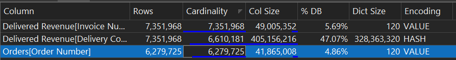
Order Number and Invoice Number both have a very high cardinality and seem to be unique for their respective fact tables.
4. Do large columns have the expected data types?
In our model the data types appear mostly as expected, but we notice that we have ‘Double’ and never fixed decimal data types. We also have a lot of ‘DateTime’ fields, but no ‘Date’ fields. If we check a few of these fields, though, we see that the time is always midnight, so there is no time data being stored in this model, that we can see, yet.
5. Do large columns have the expected dictionary size and encoding?
In 2-3 we observed that [Net Invoice Value] and [Delivery Cost] do not have the expected encoding. This is something to pay attention to when we later optimize the model.
6. Are there tables with atypically more columns than usual (usually > 10-15 columns is a flag)?
Our fact tables have an atypically large number of columns: 13 and 20 for orders and revenue, respectively. Likely, some of those columns could be turned to measures, or are not necessary for our reporting purposes. Regardless, it’s good to check what they each are so we are aware.
It seems the main reason for this is that we have a number of different fact and date fields, and a few small string fields that flag certain groups of rows.

There are a bunch of dates in our fact tables
7. Are there relationships with RI violations?
We can see that one table has 3 RI violations that are mapping to the ‘Date’ table. It seems there are problems with the relationships between our ‘Date’ dimension table and the other fact tables. Since we see in the ‘Relationships’ view these relationships are many (fact) to one (‘Date’) with bidirectional filtering disabled, then it means our fact tables have date keys not present in our date table, resulting in the RI violation.
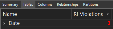
There are 3 RI violations from the Date table.
8. How much, how severe & what are some sample violations of the missing keys?
When we look at the data we can clearly see where the RI Violation comes from. There are 2 active relationships from the ‘Date’ table: one to the ‘Delivered Revenue’[Billing Date] and another to ‘Orders’[Order Date]. There is also an inactive relationship from ‘Date’[Date] to ‘Orders’[Requested Goods Receipt Date]. All of these have 365 missing keys; there appears to be a year missing from our ‘Date’ dimension table. We can confirm this because the ‘Sample Violations’ show us 3 examples - the first in the list, the middle, and the last, all of which are in 2018 (Jan 1, July 2, Dec 31).
Note that the RI Violations are counting not only for active, but also inactive relationships. If you are observing RI violations in your model, this can be a handy way to find out that your inactive relationships are causing those (Blank) values in slicers, filters or visuals.

There seems to be 2018 missing from the ‘Date’ table, causing the RI violations
9. How is the data partitioned, and do we observe the expected segment size?
The last thing we can check is how the data is stored. We see that there is no incremental refresh, nor custom partitioning of the data; each table has 1 partition. That is useful to know, because if refresh time is a complaint, then we already know that incremental refresh could be an option to speed up refresh times. What else is interesting is that we have 8 segments in the ‘Delivered Revenue’ table, and 6 segments in the ‘Orders’ table. A quick check at their rowcount and we can see the segment size is 1M. So we also know that Large Dataset Storage Mode is not enabled on the service. Since Large Dataset Storage mode has a segment size of 8M rows, we might hypothesize that enabling it and reducing the # segments could be a potential avenue to explore for further optimization, as there will be less parallel operations at query time.

There are no custom partitions, and the segment size is ~1M, not 8M (Large dataset storage mode not enabled)
With little effort, we have found several large, potential optimizations in our model.
Round the [Delivery Cost] column in the ‘Delivered Revenue Table’
Remove the [Net Invoice Value] column in the ‘Delivered Revenue' table, replacing the logic with a SUMX DAX measure.
Remove the Invoice & Order number columns, which are not in reports or used, presently
Revise the ‘Date’ table to include the year 2018, or filter 2018 data if it’s not needed.

Removing 3 columns, revising 1 column, 1 table and several measures - the model size went from 821MB to 259MB; almost 70% smaller.
There’s even more we could do — this is just a start.
Step 6: Export the results
We have done our analysis and now must document the results. We can easily do this if we export results as a .vpax file, by clicking the ‘Export’ button, at the top. we can open it for later viewing in Tabular Editor 3 (with the ‘Import’ button), DAX Studio, or the VertiPaq .xlsm (for example if we want to do further analysis in Excel or make a Power BI report on the results).
One useful feature is that the .vpax export will also by default include information about the tabular object model (model metadata) which gives context to the analysis done. That way, if a dataset goes through multiple iterations and analyses, you can always revisit prior ones with the context from the model metadata, at the time of analysis. Note that the data itself is not included in this .vpax storage, only the summary statistics and model metadata. This is obviously very helpful; conducting reproducible and well-documented analyses is an essential practice.
VertiPaq Analyzer: a first good step in every dataset analysis
VertiPaq Analyzer is a helpful tool for data-driven exploration of a tabular model.
The information from the Analyzer are derived from the model DMVs.
The main use-cases are for performance optimization by optimizing (reducing) model size & relationship size/integrity.
It provides summary statistics about objects & their in-memory size, as well as relationship RI violations, their magnitude and samples.
The VertiPaq Analyzer is easy to use, but understanding & interpreting the results of the Analyzer can be the hardest part. Each field is defined above, with some extra info.
Some typical things to look out for:
Columns & Tables that are outliers in size, cardinality or row count
Columns that have unexpected encoding and/or data types
The number, origin and impact of RI violations
How the data is partitioned and what the segment size is
We should export our results for documentation & reproducibility, and can view them, later.
For more about VertiPaq: Check out the articles & videos by sqlbi, as well as their DAX Tools video course.
For more about Tabular Editor 3: I have a series running weekly with new TE3 articles & tutorials.
NEXT UP: QUERY DMVs FOR HELPFUL MODEL INFO.
In the next article of this series, we dive deeper into the Dynamic Management Views used by the VertiPaq Analyzer to give us our results. We look at the use-cases for DMVs, and how to query these DMVs from TE3 yourself, to explore and document other aspects of our model like measures, Power Query, and more.
This will serve as an introduction to the final part, where we exploit these DMVs ourselves in C# scripts & macros of TE3, to simplify documentation & detection of data issues.
Click here for the next article in the series